The R language is very good for statistical computations, due to its strong functional capabilities, its open source philosophy, and its extended package ecosystem. However, it can also be quite slow, because of some design choices (e.g. lazy evaluation and extreme dynamic typing).
This tutorial is mainly based on Hadley Wickam’s book Advanced R.
Before optimising…
First of all, before we start optimising our R code, we need to ask ourselves a few questions:
-
Is my code doing what I want it to do?
-
Do I really need to make my code faster?
-
Is considerable speed up even possible?
For the first point, is to useful to keep the following quote in mind:
Premature optimisation is the root of all evil. (Donald Knuth)
When writing code, we have a specific task in mind, and this has to be our main focus. To make our lives simpler, it is important to write simple, understandable code to start with; it is considerably easier to debug simple code than complex code. Only when we are certain that our code is correct can we turn to the next point.
An R script that will be used only once does not necessarily need to be optimised, and writing your code quickly will probably be more important than writing code that runs quickly.
Finally, when your code is bug-free and you do need to make it faster, you need to identify the bottle-necks, the places where your code spends the most time, and you need a way to compare the speed of multiple expressions. These two things are known as profiling and benchmarking; we will treat them both in what follows.
Benchmarking
There are a few ways to time your code. The simplest is to use the function system.time():
system.time(x <- runif(10^6))
## utilisateur     système      écoulé
##        0.10        0.01        0.11
However, this timing will depend on your OS, it will generally differ from one run to the other, and therefore it is not clear how to use it to compare two or more expressions. Nonetheless, it is probably the way to go when you want to time expressions that take a long time to run.
For comparisons, we will use the microbenchmark package. Its microbenchmark function will run a series of expressions multiple times and return a distribution of running times. It can also be used with ggplot2 to output a nice graphical display of the comparisons.
library(microbenchmark); library(ggplot2)
# Create a dataframe with random values
data <- data.frame("column1" = runif(1000),
                   "column2" = rnorm(1000))

# Extract the first entry of the 666th row
compare <- microbenchmark::microbenchmark( "extract1" = {
  data[666, 1]
}, "extract2" = {
  data[[1]][666]
})

compare
## Unit: microseconds
##      expr    min      lq     mean  median      uq    max neval
##  extract1 22.021 22.9945 24.74206 23.2465 23.7395 98.219   100
##  extract2 10.384 11.3535 13.13219 12.3750 12.8605 57.486   100
ggplot2::autoplot(compare)
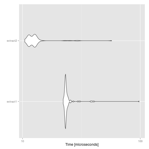
So we compared two ways of extracting an element in the data frame: first, we think of data as being matrix-like and extract based on its row and column position; or we remember that data frames are actually lists and extract the element by using the list methods. As we can see, the latter is about twice faster than the former. However, by looking at the units (i.e. microseconds), we see that the difference is quite minimal and unlikely to improve your code (unless you perform this operation millions of times).
The microbenchmark function is the main tool we will use below to benchmark snippets of code and, most importantly, compare different implementations of a same idea.
Before going into profiling…
As I mentionned above, R has the reputation of being slow. However, we have to keep in mind that most of the time, slow R code can be made faster by simply coding in a way that is more natural for R. And to understand what is natural, we need to understand a bit more about how R works.
R is an interpreted language
This means that the R interpreter translates our script into small chunks of pre-compiled code. The most common implementation of R is coded using about 50% of C code and 25% of FORTRAN code.
Vectorization is a way of coding in R which tries to make the best use of the pre-compiled code. The main idea is to code in such a way that our computations are done on vectors instead of numbers. We will look at two examples.
First, let’s say we want to compute the sum of all pairs of positive integers from 1 to 100. We could do this using a double loop, or in a vectorized way, using the outer function:
numbers <- 1:100

compare <- microbenchmark::microbenchmark("2loops" = {
  for(i in numbers) {
    for(j in numbers) {
      i + j
    }
  }
}, "vect" = {
  outer(numbers, numbers, `+`)
})

compare
## Unit: microseconds
##    expr      min        lq       mean    median        uq      max
##  2loops 3030.975 3093.1255 3324.46216 3159.6165 3231.6265 5304.771
##    vect   79.854   82.4825   95.66377   92.1305  104.1775  162.883
##  neval
##    100
##    100
ggplot2::autoplot(compare)
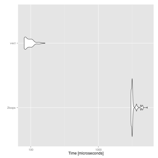
There is a 40-fold difference between the two expressions!
As a second example, let’s compute the mean across all rows of a matrix. We will do it using three different approaches: a for loop, using the apply function, and using the rowMeans function:
mat <- matrix(rnorm(20*100), nrow=100, ncol=20)

compare <- microbenchmark::microbenchmark("loop" = {
  for(i in 1:nrow(mat)) {
    mean(mat[i,])
  }
}, "apply" = {
  apply(mat, 1, mean)
}, "rowMeans" = {
  rowMeans(mat)
})

compare
## Unit: microseconds
##      expr     min       lq      mean  median       uq      max neval
##      loop 746.423 766.4940 851.05493 788.150 864.4910 3047.323   100
##     apply 863.475 883.7845 923.21638 899.168 945.9720 1084.456   100
##  rowMeans  18.150  19.2530  22.51806  22.703  24.4285   34.650   100
ggplot2::autoplot(compare)
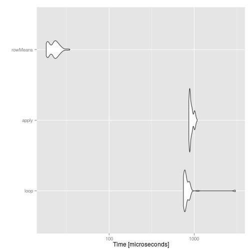
Again, we see close to a 40-fold difference.
What vectorization does is essentially moving the for loop from R to C. Moreover, the function apply is simply a wrapper for a loop, and this is why it is usually as fast as a loop (in this example, it is actually slower than a loop, because we are not recording the results of the loop but apply is).
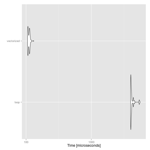
Let’s look at another example:
# Create a vector of values
categories <- c("Low", "Middle", "High")

values <- sample(categories, size = 1000, replace = TRUE)

# Change the vector of values to numeric
# 1. Using a loop
values_num1 <- rep_len(NA, length(values))
for (i in 1:length(values_num1)) {
  if (values[i] == "Low") values_num1[i] <- 0
  if (values[i] == "Middle") values_num1[i] <- 1
  if (values[i] == "High") values_num1[i] <- 2
}

# 2. Using vectorization
values_num2 <- 1 * as.numeric(values == "Middle") +
  2 * as.numeric(values == "High")

identical(values_num1, values_num2)
## [1] TRUE
# Compare the two implementations
library(ggplot2); library(microbenchmark)

compare <- microbenchmark("loop" = {
  values_num1 <- rep_len(NA, length(values))
  for (i in 1:length(values_num1)) {
    if (values[i] == "Low") values_num1[i] <- 0
    if (values[i] == "Middle") values_num1[i] <- 1
    if (values[i] == "High") values_num1[i] <- 2
  }
}, "vectorized" = {
  values_num2 <- 1 * as.numeric(values == "Middle") + 2 * as.numeric(values == "High")
})

compare
## Unit: microseconds
##        expr      min       lq      mean   median       uq      max
##        loop 3991.204 4023.503 4198.8841 4053.097 4149.492 5594.456
##  vectorized  105.098  106.666  110.4647  111.180  113.387  131.265
##  neval
##    100
##    100
autoplot(compare)
R is a dynamic language
Unlike C/C++, objects in R can change quite a lot during a computation: data frames can become matrices, we can flatten lists and create atomic vectors, the class of an object can be modified multiple times, etc. This flexibility, however, usually comes with a computational cost. For example, most functions you can find in packages will perform “input checking” to control the behaviour. Understanding R coercion rules can sometimes lead to faster (and more predictable) code.
For example, the function sapply will apply a function to each element of a list and try to simplify the input to an array. However, if simplification is not possible, it will output a list without any warning. For this reason, it is preferable to use vapply, which takes one more argument: an example of desired output.
foo <- list(c(1,2,3,4), c(1,1,2,3,4))

sapply(foo, Filter, f = function(t) t == 1)
## [[1]]
## [1] 1
##
## [[2]]
## [1] 1 1
vapply(foo, Filter, f = function(t) t == 1, 1L)
## Error in vapply(foo, Filter, f = function(t) t == 1, 1L): values must be type 'integer',
##  but FUN(X[[1]]) result is type 'double'
Because we are telling vapply what type of output we expect, this can actually lead to faster code:
fits <- lapply(1:100, function(t) {
  lm(rnorm(100) ~ rnorm(100, 2))
})

compare <- microbenchmark("sapply" = {
  sapply(fits, coef)
}, "vapply" = {
  vapply(fits, coef, c(1.0, 1.0))
})

compare
## Unit: microseconds
##    expr     min       lq     mean  median       uq      max neval
##  sapply 596.619 621.1735 650.6462 638.453 682.5425  919.996   100
##  vapply 516.375 540.4710 583.9992 562.221 594.6660 2332.687   100
autoplot(compare)
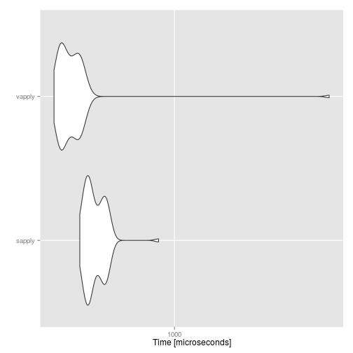
For this example, the efficiency gain is minimal. As another example, imagine you want to make sure that when you select columns of a matrix, you still get a matrix and not an atomic vector (when subsetting, R will by default coerce a matrix with one row or one column to a vector). You can coerce the result to a matrix, or use the (little known) drop argument of the function [:
mat <- matrix(rnorm(20*100), nrow=100, ncol=20)

compare <- microbenchmark("coerce" = {
  as.matrix(mat[,1])
}, "drop" = {
  mat[,1,drop=FALSE]
})

compare
## Unit: microseconds
##    expr    min     lq     mean  median     uq    max neval
##  coerce 12.001 12.314 14.09449 12.5650 12.913 54.198   100
##    drop  2.424  2.751  3.08146  3.0085  3.239 11.422   100
autoplot(compare)
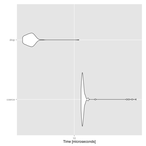
There is an 8-fold difference between the two methods. We would still need to check if the two methods give the same result:
identical(as.matrix(mat[,1]), mat[,1,drop=FALSE])
## [1] TRUE
Memory allocation
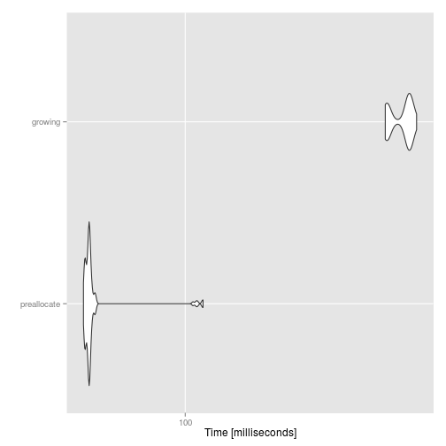
Somewhat related to the dynamism of R is the fact that memory can be frequently re-allocated during your computations, and this can lead to decrease in performance. For example, it is better to pre-allocate a vector for the results of a computation than use a for loop to continually grow the results:
compare <- microbenchmark("preallocate" = {
  results <- rep(NA, 10000)
  for(i in 1:length(results)) {
    results[i] <- runif(1)
  }
}, "growing" = {
  results = NULL
  for(i in 1:10000) {
    results <- c(results, runif(1))
  }
})

compare
## Unit: milliseconds
##         expr       min        lq      mean    median        uq
##  preallocate  53.61208  54.54148  57.95674  55.47454  55.86745
##      growing 340.49902 344.88623 375.49227 391.02795 395.07053
##       max neval
##  111.5387   100
##  412.6016   100
autoplot(compare)
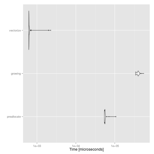
Of course, this is a silly example, because we could simply use the vectorised form runif(10000):
compare <- microbenchmark("preallocate" = {
  results <- rep(NA, 10000)
  for(i in 1:length(results)) {
    results[i] <- runif(1)
  }
}, "growing" = {
  results = NULL
  for(i in 1:10000) {
    results <- c(results, runif(1))
  }
}, "vectorize" = {
  results = runif(10000)
  })

autoplot(compare)
For other examples of what to do and what not to do, I recommend the book R Inferno. For example, memory allocation is discussed in Circle 2 and vectorisation, in Circle 3.
Profiling your code
We will now assume that our code is correct (i.e. debugged) and that we are looking for bottlenecks. This process is called profiling. We will see three slightly different ways of profiling your R code: the method available in base R through the functions Rprof and summaryRprof, the proftable function from Noam Ross, and the proftools package by Luke Tierney.
The main concept behind code profiling in R is that, while the code is running, we randomly sample time points at which we check which functions are being called. This is done by the function Rprof, which records this information in a text file. We can then call the function summaryRprof, which gives a summary of this information. Let’s look at an example:
# This example is taken from the MASS package
library(MASS)

Iris <- data.frame(rbind(iris3[,,1], iris3[,,2], iris3[,,3]),
Sp = rep(c("s","c","v"), rep(50,3)))
train <- sample(1:150, 75)
table(Iris$Sp[train])
##
##  c  s  v
## 25 25 25
Rprof(tmp <- tempfile())

res <- replicate(100, expr = {
  z <- lda(Sp ~ ., Iris, prior = c(1,1,1)/3, subset = train)
  predict(z, Iris[-train, ])$class
  z1 <- update(z, . ~ . - Petal.W.)
}, simplify = FALSE)

Rprof()

summaryRprof(tmp)
## $by.self
##                        self.time self.pct total.time total.pct
## "<Anonymous>"               0.04     4.17       0.96    100.00
## "model.frame.default"       0.04     4.17       0.30     31.25
## "[.data.frame"              0.04     4.17       0.12     12.50
## "na.omit.data.frame"        0.04     4.17       0.12     12.50
## "%in%"                      0.04     4.17       0.06      6.25
## "La.svd"                    0.04     4.17       0.06      6.25
## "unique"                    0.04     4.17       0.06      6.25
## "aperm"                     0.04     4.17       0.04      4.17
## "apply"                     0.04     4.17       0.04      4.17
## "levels"                    0.04     4.17       0.04      4.17
## "lapply"                    0.02     2.08       0.96    100.00
## "lda.formula"               0.02     2.08       0.76     79.17
## "update"                    0.02     2.08       0.32     33.33
## ".External2"                0.02     2.08       0.20     20.83
## "model.matrix.default"      0.02     2.08       0.12     12.50
## "["                         0.02     2.08       0.10     10.42
## "paste"                     0.02     2.08       0.10     10.42
## ".deparseOpts"              0.02     2.08       0.06      6.25
## "sweep"                     0.02     2.08       0.06      6.25
## "[.factor"                  0.02     2.08       0.04      4.17
## "match.call"                0.02     2.08       0.04      4.17
## "rep.factor"                0.02     2.08       0.04      4.17
## "as.integer"                0.02     2.08       0.02      2.08
## "as.matrix"                 0.02     2.08       0.02      2.08
## "c"                         0.02     2.08       0.02      2.08
## "colnames"                  0.02     2.08       0.02      2.08
## "colSums"                   0.02     2.08       0.02      2.08
## "delete.response"           0.02     2.08       0.02      2.08
## "is.finite"                 0.02     2.08       0.02      2.08
## "is.ordered"                0.02     2.08       0.02      2.08
## "lengths"                   0.02     2.08       0.02      2.08
## "match.fun"                 0.02     2.08       0.02      2.08
## "mean.default"              0.02     2.08       0.02      2.08
## "min"                       0.02     2.08       0.02      2.08
## "mode"                      0.02     2.08       0.02      2.08
## "NextMethod"                0.02     2.08       0.02      2.08
## "parent.frame"              0.02     2.08       0.02      2.08
## "sys.function"              0.02     2.08       0.02      2.08
##
## $by.total
##                        total.time total.pct self.time self.pct
## "<Anonymous>"                0.96    100.00      0.04     4.17
## "lapply"                     0.96    100.00      0.02     2.08
## "block_exec"                 0.96    100.00      0.00     0.00
## "call_block"                 0.96    100.00      0.00     0.00
## "doTryCatch"                 0.96    100.00      0.00     0.00
## "eval"                       0.96    100.00      0.00     0.00
## "eval.parent"                0.96    100.00      0.00     0.00
## "evaluate_call"              0.96    100.00      0.00     0.00
## "FUN"                        0.96    100.00      0.00     0.00
## "handle"                     0.96    100.00      0.00     0.00
## "in_dir"                     0.96    100.00      0.00     0.00
## "local"                      0.96    100.00      0.00     0.00
## "process_file"               0.96    100.00      0.00     0.00
## "process_group"              0.96    100.00      0.00     0.00
## "process_group.block"        0.96    100.00      0.00     0.00
## "replicate"                  0.96    100.00      0.00     0.00
## "sapply"                     0.96    100.00      0.00     0.00
## "try"                        0.96    100.00      0.00     0.00
## "tryCatch"                   0.96    100.00      0.00     0.00
## "tryCatchList"               0.96    100.00      0.00     0.00
## "tryCatchOne"                0.96    100.00      0.00     0.00
## "withCallingHandlers"        0.96    100.00      0.00     0.00
## "withVisible"                0.96    100.00      0.00     0.00
## "lda.formula"                0.76     79.17      0.02     2.08
## "lda"                        0.76     79.17      0.00     0.00
## "lda.default"                0.34     35.42      0.00     0.00
## "update"                     0.32     33.33      0.02     2.08
## "model.frame.default"        0.30     31.25      0.04     4.17
## "update.default"             0.30     31.25      0.00     0.00
## ".External2"                 0.20     20.83      0.02     2.08
## "predict"                    0.18     18.75      0.00     0.00
## "predict.lda"                0.18     18.75      0.00     0.00
## "[.data.frame"               0.12     12.50      0.04     4.17
## "na.omit.data.frame"         0.12     12.50      0.04     4.17
## "model.matrix.default"       0.12     12.50      0.02     2.08
## "model.matrix"               0.12     12.50      0.00     0.00
## "na.omit"                    0.12     12.50      0.00     0.00
## "["                          0.10     10.42      0.02     2.08
## "paste"                      0.10     10.42      0.02     2.08
## "match"                      0.10     10.42      0.00     0.00
## "tapply"                     0.10     10.42      0.00     0.00
## "deparse"                    0.08      8.33      0.00     0.00
## "diag"                       0.08      8.33      0.00     0.00
## "svd"                        0.08      8.33      0.00     0.00
## "%in%"                       0.06      6.25      0.04     4.17
## "La.svd"                     0.06      6.25      0.04     4.17
## "unique"                     0.06      6.25      0.04     4.17
## ".deparseOpts"               0.06      6.25      0.02     2.08
## "sweep"                      0.06      6.25      0.02     2.08
## "scale"                      0.06      6.25      0.00     0.00
## "scale.default"              0.06      6.25      0.00     0.00
## "simplify2array"             0.06      6.25      0.00     0.00
## "aperm"                      0.04      4.17      0.04     4.17
## "apply"                      0.04      4.17      0.04     4.17
## "levels"                     0.04      4.17      0.04     4.17
## "[.factor"                   0.04      4.17      0.02     2.08
## "match.call"                 0.04      4.17      0.02     2.08
## "rep.factor"                 0.04      4.17      0.02     2.08
## "[["                         0.04      4.17      0.00     0.00
## "[[.data.frame"              0.04      4.17      0.00     0.00
## "rep"                        0.04      4.17      0.00     0.00
## "as.integer"                 0.02      2.08      0.02     2.08
## "as.matrix"                  0.02      2.08      0.02     2.08
## "c"                          0.02      2.08      0.02     2.08
## "colnames"                   0.02      2.08      0.02     2.08
## "colSums"                    0.02      2.08      0.02     2.08
## "delete.response"            0.02      2.08      0.02     2.08
## "is.finite"                  0.02      2.08      0.02     2.08
## "is.ordered"                 0.02      2.08      0.02     2.08
## "lengths"                    0.02      2.08      0.02     2.08
## "match.fun"                  0.02      2.08      0.02     2.08
## "mean.default"               0.02      2.08      0.02     2.08
## "min"                        0.02      2.08      0.02     2.08
## "mode"                       0.02      2.08      0.02     2.08
## "NextMethod"                 0.02      2.08      0.02     2.08
## "parent.frame"               0.02      2.08      0.02     2.08
## "sys.function"               0.02      2.08      0.02     2.08
## "as.vector"                  0.02      2.08      0.00     0.00
## "formals"                    0.02      2.08      0.00     0.00
## ".getXlevels"                0.02      2.08      0.00     0.00
## "match.arg"                  0.02      2.08      0.00     0.00
## "model.frame"                0.02      2.08      0.00     0.00
## "nlevels"                    0.02      2.08      0.00     0.00
## "stopifnot"                  0.02      2.08      0.00     0.00
## "structure"                  0.02      2.08      0.00     0.00
## "table"                      0.02      2.08      0.00     0.00
## "vapply"                     0.02      2.08      0.00     0.00
## "var"                        0.02      2.08      0.00     0.00
##
## $sample.interval
## [1] 0.02
##
## $sampling.time
## [1] 0.96
There are two main components to this summary:
-
by.self, which represents the time spent in the function alone. -
by.total, which represents the time spent in the function, and all other functions it called.
Note that we have wrapped the code in a call to replicate, as suggested by the documentation, since its running time is very small. This is actually part of the profiling, and therefore makes it even more difficult to understand the output. This is why I recommand using Noam Ross’s proftable function. It takes the text file created by Rprof, but summarizes it differently:
proftable(tmp)
##  PctTime
##  4.17
##  4.17
##  4.17
##  4.17
##  2.08
##  2.08
##  2.08
##  2.08
##  2.08
##  2.08
##  Call
##  lda > lda.formula > model.frame.default > .External2 > na.omit > na.omit.data.frame
##  predict > predict.lda > apply
##  predict > predict.lda > scale > scale.default > sweep > aperm
##  update > update.default > lda > lda.formula > lda.default > svd > La.svd
##  lda > lda.formula
##  lda > lda.formula > model.frame.default
##  lda > lda.formula > model.frame.default > .External2 > [.data.frame > [
##  lda > lda.formula > model.frame.default > .External2 > [.data.frame > [ > [.factor
##  lda > lda.formula > model.frame.default > .External2 > na.omit > na.omit.data.frame > [ > [.data.frame
##  lda > lda.formula > model.frame.default > .External2 > na.omit > na.omit.data.frame > [[ > [[.data.frame
##
## Parent Call: local > eval.parent > eval > eval > eval > eval > <Anonymous> > process_file > withCallingHandlers > process_group > process_group.block > call_block > block_exec > in_dir > <Anonymous> > evaluate_call > handle > try > tryCatch > tryCatchList > tryCatchOne > doTryCatch > withCallingHandlers > withVisible > eval > eval > replicate > sapply > lapply > FUN > ...
##
## Total Time: 0.96 seconds
## Percent of run time represented: 29.2 %
First of all, we can see that the call to replicate is now relegated to the end and removed from the general summary. Second, we see the chain of calls, which helps us understand what some functions we didn’t call directly (e.g. .getXlevels or model.frame.default) actually do. Finally, it only shows the first few lines, ordered by their percentage of the whole running time, and therefore it is easier to read. For all these reasons, I recommend the use of proftable over summaryRprof.
There exist also graphical ways of representing the call stack. One example is the proftools package. Note that it requires the graph and Rgraphviz packages, which are available on Bioconductor.
library(proftools)
library(graphics)

Rprof(tmp <- tempfile())
# Clustering example
test.data <- function(dim, num, seed=12345) {
   set.seed(seed)
   matrix(rnorm(dim * num), nrow=num)
}
m <- test.data(120, 4500)

hclust(dist(m))
##
## Call:
## hclust(d = dist(m))
##
## Cluster method   : complete
## Distance         : euclidean
## Number of objects: 4500
Rprof()

plotProfileCallGraph(readProfileData(tmp),
                     score = "total")
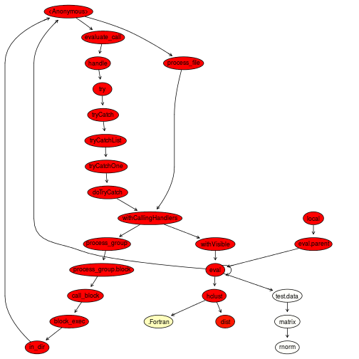
The colours are used to represent the amount of time used by each function. As we can see, the dist function is the real bottleneck in this example, and therefore improving the running time would necessitate a faster algorithm for computing the Euclidean distance.
We can see all these functions being used in a real-life example, where I tried to optimise the main component of the function which computes the PCEV in order to speed up my simulations. Follow the link to see the different steps I took.
Other things to keep in mind
Profiling the code is the best way to identify bottleneck, but it doesn’t directly tell us how to optimise our code. Below, I give three general ideas to keep in mind.
A faster implementation
The greatest strength of R is its massive package ecosystem. Often, we don’t need to write from scratch the code for a new method appearing in a paper because its authors have already published a package. Moreover, different packages may have different implementations of a same (or similar) method. This means that, sometimes, a faster implementation (or even a more efficient algorithm) can be used simply by changing the function call. One example of this is the slanczos function in the mgcv package: it computes the eigenvectors of a square matrix using a different algorithm than the one used by eigen. One advantage of this particular algorithm is its iterative nature: eigenvectors are computed one at a time, and therefore if we only need the eigenvector corresponding to the largest eigenvalue, it is possibly faster to use slanczos than eigen; from experience, I would say that this depends a lot on the size of the matrix and how many eigenvectors you need.
The next example is related to our discussion of design choices for R. R implements what is called modify-on-copy, which means that when we modify an object a (possibly partial) copy is made. For example, when we write
x <- x[,c(1,2,4)]
the result of subsetting x on its columns is stored in a temporary variable, which is then assigned x (and in fact, this is what allows us to use x on both sides of the assignment operator). This allows for clearer code, but it actually slows down the execution and can lead to quite a lot of memory being used (this is why it is usually suggested to fill your memory only up to one third of its capacity, leaving space for all these copies).
Enter the package data.table. For large datasets, it can be significantly faster (i.e. several orders of magnitude) than using a plain data frame. Its speed comes from a new implementation of the usual data frame routines (e.g. rbind, subset, etc.) using a pass-by-reference syntax; in other words, no copy of the data is made during modification (although this behaviour can actually be broken if not used properly).
Byte-code compilation
Recall from above that R is an interpreted language. The code we run has to be decomposed in small parts (called token) which are then mapped to pre-compiled code. One way to speed up your code is therefore to do this mapping once and for all for functions (or expressions) that are used quite often; this can be done using the compiler package (which is now part of the standard packages you get by default).
library(compiler)

# Original implementation of lapply
old_lapply <- function(X, FUN, ...) {
   FUN <- match.fun(FUN)
   if (!is.list(X))
    X <- as.list(X)
   rval <- vector("list", length(X))
   for(i in seq(along = X))
    rval[i] <- list(FUN(X[[i]], ...))
   names(rval) <- names(X)
   return(rval)
}

old_lapply_comp <- cmpfun(old_lapply)

data <- lapply(1:1000, function(i) rnorm(100))

compare <- microbenchmark("original"=old_lapply(data, mean),
                          "compiled"=old_lapply_comp(data, mean),
                          "new"=lapply(data,mean), times=1000)
compare
## Unit: milliseconds
##      expr      min       lq     mean   median       uq      max neval
##  original 8.540425 8.810987 9.203373 8.906748 8.999030 95.57505  1000
##  compiled 6.803040 7.028638 7.291496 7.102944 7.204534 15.12300  1000
##       new 6.009491 6.229223 6.523165 6.306225 6.393313 90.89608  1000
autoplot(compare)
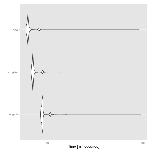
As we can see, byte-code compilation actually improves speed, even though the new implementation is even faster. Similarly, expressions can be compiled using the function compile, and the result can be evaluated using eval:
expr <- compile(rev(1:100) + 1:100)
eval(expr)
To see how the compiler package can be used to turn the usual interpreter into a “just-in-time” compiler, see the following blog post.
Concluding remarks
In this tutorial, we first discussed why you would want to optimise your code, and how to keep in mind some of the key features of R so that the code you write in the first place isn’t too bad. We then showed how to benchmark pieces of code, and how to use some of the many profiling resources out there.
This is not the end of the discussion. Two main points I didn’t discuss are how to incorporate low-level languages (e.g. C, C++, Fortran) in your code, and how to take advantage of multiple cores to do parts of the computations in parallel. These two points are already well covered in some other places, like here and here.
Finally, two more options to consider (but a lot more drastic!) are to either link your version of R to a different, more efficient BLAS (Basic Linear Algebra System), or even to go for a faster R implementation (e.g. pretty quick R or Renjin). However, I haven’t tried either option, and therefore I cannot comment on them.
In conclusion, another quote from Donald Knuth (pointed out by Vince Forgetta):
If you optimize everything, you will always be unhappy. (Donald Knuth)
Update (2015-10-15): I’ve actually switched to the ATLAS system a few weeks ago, and the improvements I got are similar to the results discussed in the link above. For Ubuntu users, I recommend to make the switch, since there doesn’t seem to be any downside!