Multivariate t distribution

I am currently teaching a graduate course in Multivariate Analysis (the course website can be found here). A few weeks ago, I introduced the family of elliptical distributions. In this blog post, I want to discuss the multivariate t distribution, how to generate samples, and highlight the issue of uncorrelatedness vs independence.

Elliptical distributions

If we generate samples from a multivariate normal, we can easily see that the contour lines are ellipses:

set.seed(7200)
library(mvtnorm)

n <- 10000
p <- 2
Sigma <- matrix(c(1, 0.5, 0.5, 1), ncol = p)
Y <- data.frame(rmvnorm(n, sigma = Sigma))

# Plot the data
library(ggplot2)

ggplot(Y, aes(X1, X2)) + 
  geom_point(alpha = 0.2) +
  geom_density_2d() +
  theme_minimal()

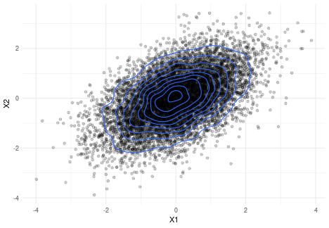
Elliptical distributions are a generalization of the multivariate normal distribution that retain this property that lines of constant density are ellipses.

There are many ways to formalise this definition. For example, let $\mu\in\mathbb{R}^p$ and $\Lambda$ be a $p\times p$ positive-definite matrix. If $\mathbf{Y}$ has density

$$f(\mathbf{Y}) = \lvert\Lambda\rvert^{-1/2}g\left((\mathbf{Y} - \mu)^T\Lambda^{-1}(\mathbf{Y} - \mu)\right),$$

where $g:[0, \infty)\to [0, \infty)$ does not depend on $\mu,\Lambda$, we say that $\mathbf{Y}$ follows an elliptical distribution with location-scale parameters $\mu,\Lambda$, and we write $\mathbf{Y}\sim E_p(\mu,\Lambda)$.

We can recover the multivariate normal distribution by taking $g(u) = (2\pi)^{-p/2}\exp\left(-\frac{1}{2}u\right)$.

Multivariate t distribution

One very important example of elliptical distribution is the multivariate t distribution. Its density is defined as follows: if we let $\nu > 0$, we have

$$f(\mathbf{Y}) = c_{p,\nu}\lvert\Lambda\vert^{-1/2}(1 + (\mathbf{Y} - \mu)^T\Lambda^{-1}(\mathbf{Y} - \mu)/\nu)^{-(\nu+p)/2},$$

where

$$c_{p,\nu} = \frac{(\nu\pi)^{-p/2} \Gamma\left(\frac{1}{2} (\nu + p)\right)}{\Gamma\left(\frac{1}{2}\nu\right)}.$$

This clearly fits our definition of an elliptical distribution: simply take $$g(u) = c_{p,\nu}(1 + u)^{-(\nu+p)/2}.$$

There is a different, equivalent way of defining the multivariate t distribution: let $W$ be such that $\nu W^{-1}\sim\chi^2(\nu)$, and let $\mathbf{Z} \sim N(0, I_p)$. Then we have

$$\mu + \sqrt{W}\Lambda^{1/2}\mathbf{Z} \sim t_{p,\nu}(\mu, \Lambda).$$

This representation readily gives us a way to generate samples from a t distribution.

Generating samples

So the equation above gives us a recipe for generating a sample $\mathbf{Y}_1, \ldots, \mathbf{Y}_n$: for $i=1, \ldots, n$:

1. Generate $X_i\sim \chi^2(\nu)$ and set $W_i = \nu/X_i$;
2. Generate $\mathbf{Z}_i\sim N(0, I_p)$ (e.g. by generating $p$ univariate standard normal variables);
3. Set $\mathbf{Y}_i = \mu + \sqrt{W_i}\Lambda^{1/2}\mathbf{Z}_i$.

We can easily implement this in R:

n <- 100
p <- 2 
nu <- 3
Lambda_sqrt <- expm::sqrtm(Sigma)

data <- replicate(n, {
  X <- rchisq(1, df = nu)
  W <- nu/X
  Z <- rnorm(p)
  Y <- sqrt(W) * Lambda_sqrt %*% Z
  
  return(drop(Y))
})

Of course, we can do this much more efficiently:

W <- nu/rchisq(n, df = nu)
Z <- matrix(rnorm(n*p), ncol = p)
Y <- sqrt(W) * Z %*% Lambda_sqrt

Or yet another way is to use the function mvtnorm::rmvt:

Y <- rmvt(n, df = nu, sigma = Sigma)

For more details on how to sample t variates in R, I recommend this paper by Marius Hofert.

Uncorrelated vs Independent

Students of statistics are taught the different between correlation and dependence, or between uncorrelatedness and independence: two independent variables are uncorrelated, but the converse is not true in general. Of course, the big exception is the normal distribution: two normal variables are uncorrelated if and only if they are independent. And even though elliptical distributions behave similarly to the multivariate normal distribution, this property does not translate to the rest of the elliptical distributions. Indeed, we even have the following result:

Proposition

Within the class of elliptical distributions $E_p(\mu,\Lambda)$, the property that independence and uncorrelatedness are equivalent uniquely defines the multivariate normal distribution.

This result is important! Because whereas I was able to generate a standard multivariate normal $Z$ by simply generating $p$ standard univariate normals, I cannot do the same for the uncorrelated (i.e. $\Lambda = I_p$ ) multivariate t distribution. We can clearly see how this wrong using a simulation:

library(tidyverse)
B <- 10000
nu <- 3

# Generate uncorrelated t distribution
mult_t <- rmvt(B, df = nu)
# Generate independent t distribution
indep_t <- matrix(rt(2*B, df = nu), ncol = 2)

# Create a tibble for plotting
colnames(mult_t) <- colnames(indep_t) <- c("X", "Y")

mult_t <- mult_t %>% 
  as_tibble() %>% 
  mutate(Type = "Joint T")

indep_t <- indep_t %>% 
  as_tibble() %>% 
  mutate(Type = "Indep T")

data_plot <- bind_rows(
  mult_t,
  indep_t
)

# Plot the results
data_plot %>% 
  ggplot(aes(X, Y)) + 
  geom_point(alpha = 0.2) +
  theme_minimal() +
  facet_grid(. ~ Type) +
  geom_density2d()

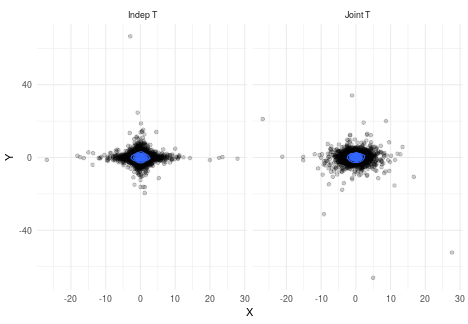
As we can see from the left panel, by multiplying two marginal t distribution, we do not get an elliptical distribution; the contour lines are closer to diamonds.