Principal Component Analysis (PCA) and classical Multidimensional Scaling (MDS) are two closely related dimension reduction methods. In fact, under certain conditions, there are exactly the same. Their main difference is the type of input they take:
- PCA: A dataset where each row is an observation, and each column is a feature.
- MDS: A distance matrix.
Let’s look at an example. We will apply PCA to the USArrests data that is included with base R. Each row is a US state, and the four columns correspond to:
- Number of arrests for murder per 100,000.
- Number of arrests for assault per 100,000.
- Number of arrests for rape per 100,000.
- Percent of the population that lives in an urban area.
For the purposes of this post, we will ignore the fact that one of the variables is measured on a different scale than the others.
We can perform PCA using the function prcomp, to which we directly pass the dataset.
# PCA on USArrests dataset
pca_out <- prcomp(USArrests)
The object pca_out now contains the information you would need to evaluate the results of this PCA decomposition. See the help page for more information.
With MDS, we need to compute the distance matrix first. Here we choose the Euclidean distance.
# Compute Euclidean distance between each observation
dmat <- dist(USArrests)
mds_out <- cmdscale(dmat, k = 4)
The function cmdscale requires both the distance matrix and the number of dimensions. Note that in PCA, we passed the full dataset, and therefore prcomp “knows” how many dimensions to consider. In MDS, we need to be explicit.
Because we chose the Euclidean distance, it turns out that PCA and MDS give us the same decomposition. We can check that this is the case as follows:
# Equality only up to a sign
# Remember: Eigenvectors are not unique!
all.equal(pca_out$x, -mds_out,
          check.attributes = FALSE)
## [1] TRUESo what is the point of MDS, if there is an extra step but we get the same output? Sometimes, all we have to work with is a distance matrix. For example, the eurodist dataset (also included with base R) contains road distances (in km) between 21 European cities. In this setting, we can perform MDS on the distance matrix and visualize the data in two dimensions.
mds_out <- cmdscale(eurodist, k = 2)

# Visualize
plot(mds_out[, 1], mds_out[, 2], type = "n",
     xlab = "MDS1", ylab = "MDS2", asp = 1)
text(mds_out[, 1], mds_out[, 2],
     rownames(mds_out), cex = 0.6)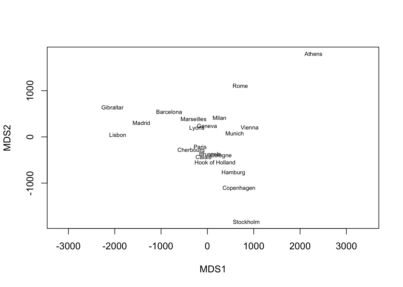
We can see from the plot that MDS recovers the geographic arrangement of European cities, with North and South flipped.
Therefore, to apply PCA, we need data in matrix form. However, to apply MDS, all we need is a distance matrix. The observations themselves could be anything: cities, DNA sequences, molecules, etc.
For more details on MDS (and its nonlinear extensions), see these slides from my Multivariate Analysis course.